Using the analysis module

The analysis module contains a small selection of useful analysis tool that can be use to extract informations from GammaSpectrum objects.

Searching peaks in a spectrum

The analysis module provides a simple peak-search function based around the scipy.signal.find_peaks function. The search is based on a user-specified prominence value.

A peak search can be easily performed giving the desired spectrum to the peak_search function specifying a prominence value. The function returns a dictionay containing as key an integer index of the peak and as values a list containing the channel index corresponding to the peak maximum, its intensity in counts per seconds per channel and, if a calibration has been applied to the spectrum, the energy value of the maximum. As an example let us apply a peak search to the \(^{226}\text{Ra}\) presented in the previous sections.

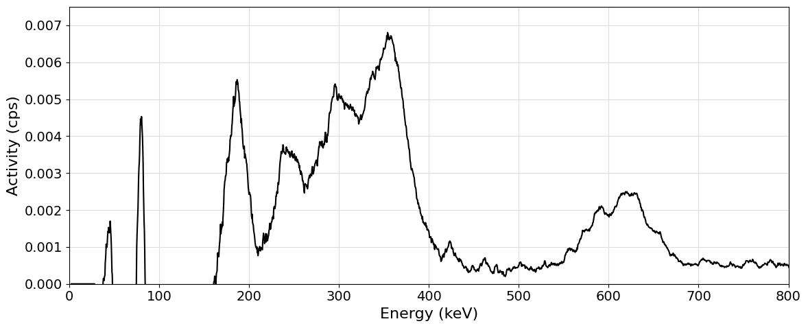
Let us load the sample and background spectra together with the calibration file and let us generated a smoothed out difference spectrum to be used in the peak search.

from pygammaspec.spectrum import GammaSpectrum, Calibration
from pygammaspec.visualization import plot_spectrum

sample = GammaSpectrum.from_PRA_histogram("../utils/weak_radium.txt", 25851)
background = GammaSpectrum.from_PRA_histogram("../utils/background.txt", 25851)
calibration = Calibration.from_calibration_file("../utils/calibration.txt")

spectrum = (sample-background).average_smoothing(10)
spectrum.calibration = calibration

plot_spectrum(spectrum, enrange=(0, 800), yrange=(0, 0.0075))

Now that the desired spectrum has been obtained let us perform a peak search using the peak_search function:

from pygammaspec.analysis import peak_search

peaks = peak_search(spectrum, prominence=0.001)

for i, (channel, counts, energy) in peaks.items():
  print(f"{i}: {energy:.2f} keV \t{counts:.2e} cps\t\t(channel: {channel:.2f})")

0: 45.60 keV 	1.70e-03 cps		(channel: 1.40)
1: 80.50 keV 	4.53e-03 cps		(channel: 2.40)
2: 186.87 keV 	5.53e-03 cps		(channel: 5.23)
3: 237.85 keV 	3.77e-03 cps		(channel: 6.49)
4: 295.81 keV 	5.41e-03 cps		(channel: 7.86)
5: 354.15 keV 	6.80e-03 cps		(channel: 9.18)
6: 620.40 keV 	2.50e-03 cps		(channel: 14.62)

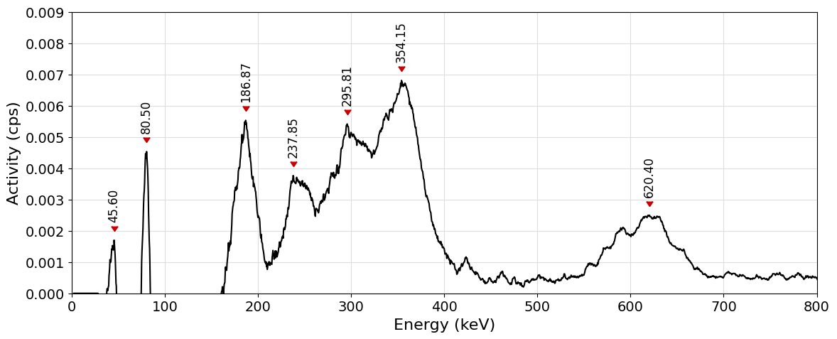
Please notice how the peak_search function is also embedded into the plot_spectrum function from the visualization module. If a prominence value is specified in the call to plot_spectrum, markers with either energy or channel values (depending on the plot mode) will be plotted on the spectra:

plot_spectrum(spectrum, enrange=(0, 800), yrange=(0, 0.009), prominence=0.001)

Fitting single peaks in the spectrum

The analysis module provides a simple peak-fit function based around the scipy.optimize.curve_fit function. The function can be used to fit peaks in a GammaSpectrum object once it has been calibrated. Given a region of initerest, the alogrithm fits the experimental datapoints with a Gaussian function of unitary height corrected by a polinomial baseline of a user-defined order \(N\). The expression of the fitting function \(f(\varepsilon)\), written in terms of the vector \(\mathbf{c}=[c_0, c_1, c_{N+3}]\) of optimized parameters, is the following:

\[ f(\varepsilon) := c_0 e^{-\frac{(\varepsilon-c_1)}{2 c_2^2}} + \sum_{n=0}^N c_{n+3} \varepsilon^n\]

where \(\varepsilon\) represents the energy in \(\text{keV}\), \(c_0\) represents the height of the gaussian fitting the peak, \(c_1\) represents the energy in \(\text{keV}\) at which the peak is located, \(c_2\) represents the standard deviation of the Gaussian while the coefficients \(\{c_3, ..., c_{N+3}\}\) represents the coefficients of the polynomial expansion.

The peak_fit function retuns many objects. In the order:

• A list of float values of length \(N+4\) representing the vector \(\mathbf{c}\) of optimized parameters

• A list of float values representing the section of energy values used in the fitting procedure.

• A list of float values containing the function profile in the considered energy region.

• A list of float values containing the baseline profile in the considered energy region.

• A float value representing the estimated efficiency of the detector on the fitted peak.

Note

The efficiency \(\eta\) of the detector is computed based on the ratio of the full-width at half maximum (\(\text{FWHM}\)) of the gaussian fitting the peak and the energy \(\varepsilon_0\) at which the peak is centered.

\[ \eta := 100\frac{\text{FWHM}}{\varepsilon_0} \]

or, in terms of the optimized coefficents:

\[ \eta = 100 \frac{2c_2\sqrt{2\ln{2}}}{c_1} \]

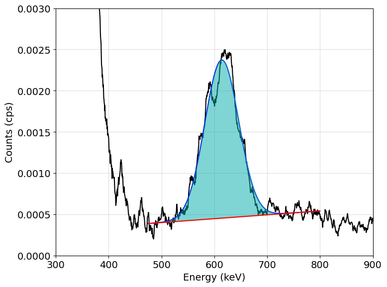
To show how the peak fitting function can be used let us consider the peak of \(^{214}\text{Bi}\) at \(609.9 \text{keV}\) in the previously obtained spectrum. Let us perform a fitting in the region from \(475\text{keV}\) to \(750\text{keV}\) using a linear baseline (order 1):

from pygammaspec.analysis import fit_peak

popt, efit, yfit, bfit, efficiency = fit_peak(spectrum, 475, 800, baseline_order=1)

print("Fitting results:")
print("----------------------------------------")
print(f"Central energy: {popt[1]:.2f} keV")
print(f"Peak height: {popt[0]:.2e} cps")
print(f"Peak STD: {popt[2]:.2f} keV^2")

Fitting results:
----------------------------------------
Central energy: 614.02 keV
Peak height: 1.92e-03 cps
Peak STD: 32.14 keV^2

The fitting results can be easily plotted using the data provided by the fitting function:

import matplotlib.pyplot as plt

fig = plt.figure(figsize=(8, 6))

plt.plot(spectrum.energy, spectrum.counts, c="black", zorder=3)
plt.plot(efit, yfit, c="blue", zorder=3)
plt.plot(efit, bfit, c="red", zorder=4)

plt.fill_between(efit, yfit, bfit, color="#00AAAA", alpha=0.5, zorder=3)

plt.xlim((300, 900))
plt.ylim((0, 0.003))

plt.xlabel("Energy (keV)", size=14)
plt.ylabel("Counts (cps)", size=14)

plt.grid(which="major", c="#DDDDDD")

plt.tight_layout()
plt.show()