Species and Auxiliary functions
The System class also supports the definition of auxiliary curves. These are combination of concentrations of various species in solution and are very useful in the solution of many different acid-base problem. For example, by using auxiliary curves, one can easily visualize the point in which the protonic balance of a given solution is satisfied. To do so, however, we must discuss how simbolic expression can be constructed in the pypH environment.
The Species objects logic
The pypH library has been developed with the logic of providing the user with an almost pen an paper experience in which expressions involving concentrations of species in solution can be treated directly in an algebric expression.
What you have seen so far in the basic plotting tutorial was the definition of an generic Acid system that takes into account all its possible deprotonation states and can be used to model its behavior in solution. This operation sets the concentration of the acid and it’s \(pKa\) allowing the generation of its logarithmic diagram.
If, however, we want to write a symbolic expression involving, for example, the concentration of a given deprotonation state, we must find an univocal way of referring to a given species derived from the acid deprotonation. This, in the pypH environment can be done using the Species class and it’s derived subclasses AcidSpecies and SpectatorSpecies objects.
To obtain the symbolic representation of a given species it is sufficient to operate using the () round bracket operator on the base Acid or Spectator class. As an example, referring to the oxalic acid case presented before, the reference to the mono-acid oxalate ion can be obtained from the Acid object by specifying the deprotonation index (1) of the species:
from pypH.acid import Acid

oxalic_acid = Acid([1.25, 4.14], 0.05)

HOx_species = oxalic_acid(1)

print(HOx_species)
print(repr(HOx_species))
$[HA^-]$
AcidSpecies[id: 0, deprot. idx: 1, name: $HA^-$]
A Species object can be summed to and subtracted from other Species and Auxiliary object leading to an Auxiliary object representing a symbolic algebric expression. As an example if we want to construct the expression \([HOx^-] + 2[Ox^{2-}]\) we can operate as follows:
from pypH.acid import Acid

oxalic_acid = Acid([1.25, 4.14], 0.05)

a = oxalic_acid(1)
b = oxalic_acid(2)

expression = a + 2.*b

print(expression)
$1.0*[HB^-]+2.0*[B^{2-}]$
Plotting an Auxiliary expression
Now that we have shown how algebric expression can be created in the pypH environment, we can now show how these expressions can be plotted onto a logarithmic diagram. To demonstrate how this can be done, let us consider a practical example: the problem of computing the \(pH\) of a \(0.01M\) diammonium phosphate \((NH_4)_2HPO_4\) solution. To do so, let us start by defining the system of acids according to:
from pypH.acid import Acid

phosphoric_acid = Acid([2.14, 7.20, 12.37], 0.01, names=["$H_3PO_4$", "$H_2PO_4^-$", "$HPO_4^{2-}$", "$PO_4^{3-}$"])
ammonium = Acid([9.24], 0.02, names=["$NH_4^+$", "$NH_3$"])
To solve the problem and compute the \(pH\) of the solution, one should consider the protonic balance that, for the system in question is represented by:
To visualze the protonic balance on the logarithmic diagram one should represents both sides of the equality in terms of an Auxiliary function object. This can be done easily by adopting what discussed in the previous paragraph.
from pypH.acid import Hydronium, Hydroxide

right_side = phosphoric_acid(3) + ammonium(1) + Hydroxide
left_side = Hydronium + phosphoric_acid(1) + 2.*phosphoric_acid(0)

print(right_side)
print(left_side)
$1.0*[PO_4^{3-}]+1.0*[NH_3]+1.0*[OH^-]$
$1.0*[H_3O^+]+1.0*[H_2PO_4^-]+2.0*[H_3PO_4]$
Where the Hydronium and Hydroxide object are pre-defined intances of the AcidSpecies class to represent the solvent derived ions \(H_3O^+\) ad \(OH^-\).
The auxiliary curves can now be added to the plot using the add_auxiliary function according to:
from pypH.system import System

system = System()

system.add(phosphoric_acid)
system.add(ammonium)

system.add_auxiliary(right_side, name="r.h.s", color="blue")
system.add_auxiliary(left_side, name="l.h.s", color="red")

system.plot_logarithmic_diagram(show_legend=True, concentration_range=(1e-6, 1.), figsize=(10, 7))
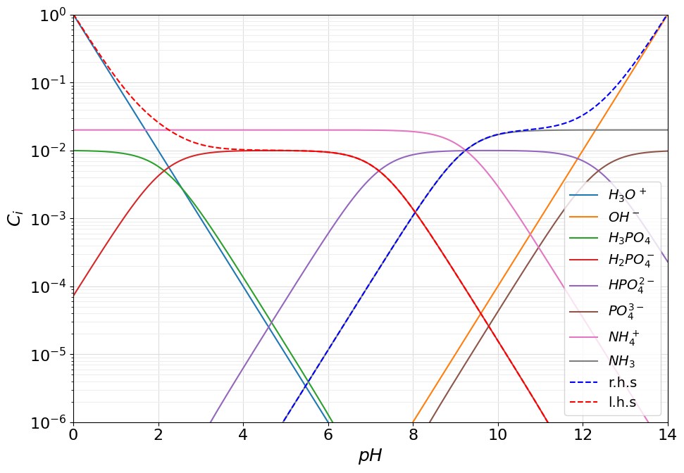
As can be seen the protonic balance is satisfied at \(pH \approx 8.05\).
Solving an auxiliary expression
In what we have shown previously the \(pH\) of a \(0.01M\) diammonium phosphate \((NH_4)_2HPO_4\) solution was deducted graphically by looking at the logarithmic diagram. The pypH library however allows also the computation of numerical solutions to the problem. To do so, the protonic balance of the system can be passed to the solve method of the System class. This function will numerically evaluate the zeros of the expression by means of the dicotomic method. The \(pH\) of the solution can, as such, be comuted according to:
computed_pH = system.solve(left_side, right_side)

print(f"The pH of the solution is {computed_pH:.4f}")
The pH of the solution is 8.0545
Very close to the value estimated before by graphical inspection.